🌐 中文版：繁體中文

Intro

Even before I started grinding LeetCode, I’d heard how terrifying DP problems are, so before actually starting on problems like these I wanted to organize my DP knowledge.

While reading material online I found this article explains it really well, so I highly recommend reading this article first. The author mentions that to understand DP, patience matters, and you also need to be comfortable with recursion, because DP problems are usually solved with recursion.

What is Dynamic Programming (DP)?

Here I have to mention the conclusion from that article: Dynamic Programming is a tool to help make recursive code more efficient. So the author also believes you shouldn’t, when facing a problem, first try to identify whether it’s a DP problem. Instead, first judge whether recursion is needed, and on top of that recursion you then think about how the recursive code might be very wasteful, so there should be room to improve the answer, and the way to improve it is through Dynamic Programming.

DP is a way to improve an existing solution!

Next I’ll introduce the steps for using this tool. There are 4 steps, and I’ll explain them step by step using one problem.

Problem: LeetCode 62. Unique Paths

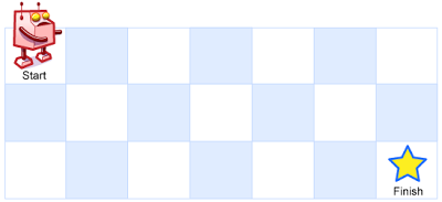
This problem gives an m x n grid with a robot at the top-left corner. Each move the robot can go down or right by one cell, and the robot tries to reach the Finish cell at the bottom-right. We need to find how many unique path combinations are possible.

Step 1: Recursion

This step is usually the most important and the key to laying out the whole solving plan. What you need to do is return to the purest central idea: recursion, which is essentially proposing a brute-force solution first.

At the same time this convinces the interviewer that you know what recursive relation this problem uses, meaning you have to find the recursive relation first before there’s room for later improvement.

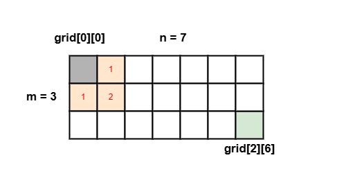
First, this problem asks how many paths can ultimately reach the end. So what do we need to know first? We need to know how many paths there are from the start to any given cell. Looking at the figure above, we can see that from the start grid[0][0] to its bottom-right cell grid[1][1] you can come from the right or from below (the problem restricts moves to right or down), two routes total, while going straight right from the start or straight down each has only one route.

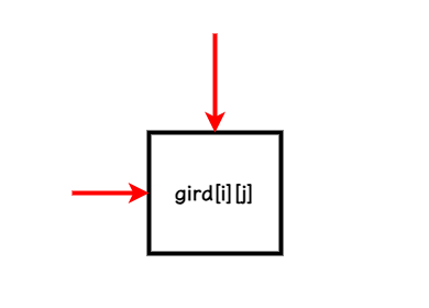
The example above should also show that for any cell [i][j], its previous step could be:

moving down from the cell above, i.e. [i-1][j]
moving over from the cell to the left, i.e. [i][j-1]

And moving one cell from above or from the left are on the same path, so the count doesn’t change. So we know that for any cell [i][j], the number of paths from the start to it is [i-1][j] + [i][j-1].

One more example also verifies this: if we want to move to grid[2][2], the total number of paths must be grid[1][2] + grid[2][1].

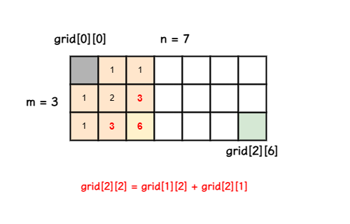
If we write the above idea as a recursion like below, the recursion’s termination condition occurs when it reaches the row right next to the start or the column below it, where it stops.

class Solution {
public:
    int uniquePaths(int m, int n) {

        if(m==1 || n==1) return 1;
        
        return uniquePaths(m-1,n) + uniquePaths(m,n-1);
    }
};

But running this you’ll find an error: Time Limit Exceeded! That means there’s something that needs improving, so on to step two.

Step 2: Recursion + Memoization

This step is where DP actually begins, but not every inefficient problem needs DP, so first weigh whether this problem is worth solving with DP. Based on the result of step one, you only need to use DP if the following conditions both hold:

Overlapping subproblems: you solve the same subproblem multiple times
An optimal substructure: by obtaining the optimal solution of each subproblem, you can get the optimal solution of the whole problem

If during an interview or while solving you find these two can’t be fully satisfied, then you shouldn’t use DP (or the approach introduced in this article). You might be able to use other techniques like backtracking instead.

So how do we confirm this problem satisfies these two conditions?

I drew the recursion tree of Step 1 below. You can see that not all subproblems actually overlap, but you can still see a lot of repeated computation, like uniquePaths(2, 6) and uniquePaths(2, 5), so it can still be seen as having overlapping subproblems.

Recursion tree of the Step 1 solution

You can zoom in to look

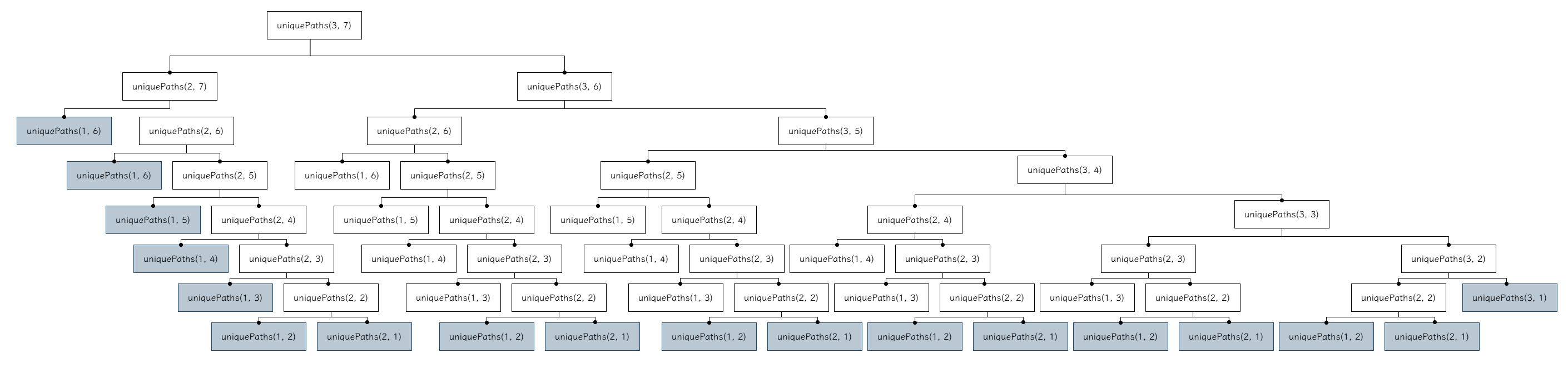
The second condition is also satisfied, because we can use [m-1][n] and [m][n-1] to get the optimal solution of [m][n].

So the goal of this step is simple: make the repeated computation happen only once, and find a way to safely store it (memoization).

The purpose of storing is to let subsequent repeated computations be conveniently looked up, reducing the amount of computation. So for the later lookups in storage, we also want to get as close to $O(1)$ complexity as possible, using an array or a hash table depending on the situation.

class Solution {
public:
    vector<vector<int>> dp;
    int helper(int m, int n){
        if(dp[m][n]){
            return dp[m][n];
        }
        else if(m==1 || n==1) {
            dp[m][n]=1;
            return dp[m][n];
        }
        
        dp[m][n] = helper(m-1,n) + helper(m,n-1);
        return dp[m][n];
    }
    int uniquePaths(int m, int n) {
        dp = vector<vector<int>>(m + 1, vector<int>(n + 1, 0));
        return  helper(m,n);
    }
};

This is the corrected result. It mainly uses a 2D vector to store the computed path counts, and since we need to initialize the array size to m+1 x n+1 (to avoid out-of-bounds access here), we split it into two functions. For this problem there aren’t many changes needed; compared to the original logic we only change two places:

store the result of a recursive call
when a recursive call already exists in the array, return the stored value (i.e. the result of helper(m,n) is already stored in dp[m][n])

Running it again now, you’ll find Submit Accepted.

And the time complexity of this run is $O(M \times N)$, which is a big efficiency boost compared to step one’s $O(2^{M+N})$ (because each level of the recursion decomposes the problem into two subproblems). Although the time complexity dropped, the space complexity used went up, but this also shows that DP is an approach that trades space for time. This is actually very worthwhile, because the space complexity of doing so is mostly linear growth, yet it can improve time complexity exponentially.

So the progress so far is: first being able to propose a brute-force recursive approach, then improving the earlier approach with extra memory! (For an interview, getting to this step is already great.)
So is there anywhere we can optimize further? That’s step three.

Step 3: Iteration + Tabulation

Normally, if there’s no obvious performance improvement in the previous step (or the interviewer wants you to improve your answer further), you’ll need step three. This step uses Tabulation rather than Memoization, and implements it with Iteration rather than Recursion.

But whether it’s Tabulation or Memoization, their goal is the same: store earlier computation results and retrieve them when they’re recomputed later.

The difference between the two is mainly in how the data is stored. Tabulation mainly stores via arrays (usually 2D arrays), while Memoization usually stores via sets, hash tables, etc. So Tabulation iterates over each array through iteration, while Memoization relies on recursive calls.

This change won’t necessarily improve time or space complexity, but the key point is: using the iterative array approach can accommodate a larger input size without being limited by the maximum call stack depth of recursive calls (too deep a call stack risks a stack overflow).

So looking back at the original Unique Paths problem, if we want to use iteration, we can iterate in reverse via a loop.

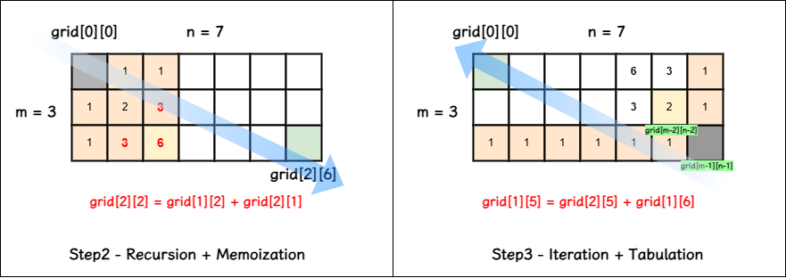
Look at the right side of this figure. In principle it walks from the bottom-right to the top-left. The reason the author chooses to start from the second-to-last row and second-to-last column cell and work backward is that the bottom row and the rightmost column all have a walkable path count of 1. So for grid[1][5], the number of steps to reach it from the new start equals grid[2][5] plus grid[1][6], giving us the relation $F(m,n) = F(m+1, n) + F(m, n+1)$.

After rewriting the program it looks like this:

class Solution {
public:
    int uniquePaths(int m, int n) {
        // init a m x n 2D vector with value 1
        vector<vector<int>> dp(m, vector<int>(n, 1));
        
        for(int i=m-2; i>=0; i--){
            for(int j=n-2; j>=0; j--){
                // do it backwardly
                dp[i][j] = dp[i+1][j] + dp[i][j+1];
            }
        }
        return dp[0][0];
    }
};

Here’s a detailed explanation of the code changes:

Declare a 2D vector of size m x n with value 1 (representing a whole grid, where the default path count is 1)
Set up loops, using the second-to-last row and second-to-last column cell ([m-2][n-2]) as the loop’s start, decrementing the index by 1 each iteration
Traverse each cell, with the rule being the relation we just derived
Iterate all the way back from the bottom-right to [0][0]; once we reach [0][0], its stored value is the total of all paths

Visualizing the traversal looks like the figure below.

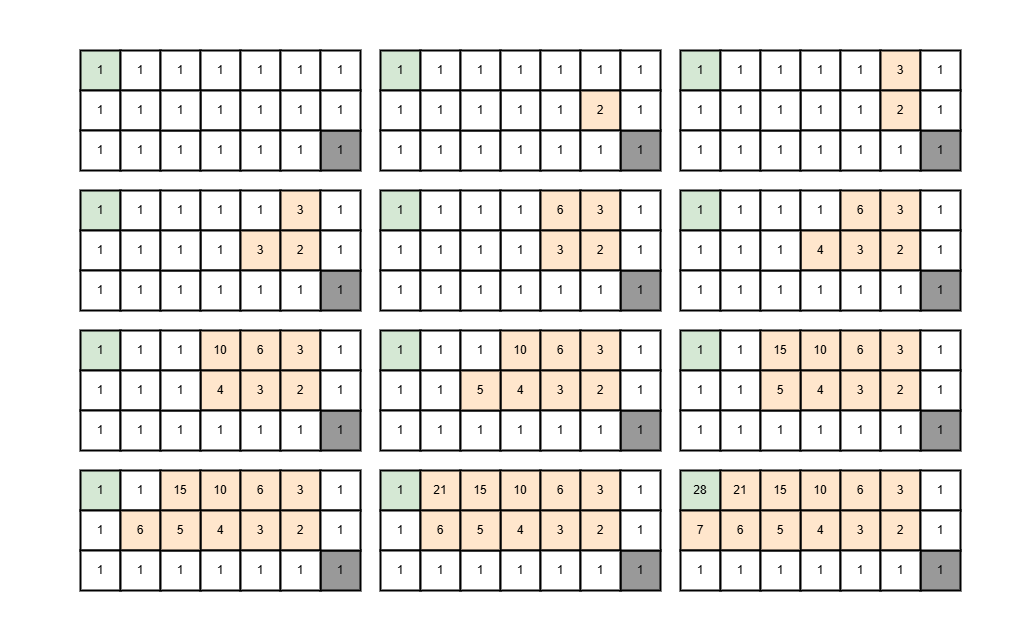
The execution result and complexity are the same as step two, and both are 100% Runtime!
The author also mentions this approach is well suited to “go from A to B” type problems, where all you have to do is fill in a table.

Step 4: Iteration + Tabulation [Optimized]

You don’t necessarily need to reach this step every time; if an interview gets through the first three steps, that’s already very good.

The goal of this step is to reduce space complexity. After the previous steps, the time complexity should already be optimized. The reason there’s still a chance to keep optimizing space complexity is that even though we earlier built an m x n grid to iteratively store the path counts, we don’t actually have to keep accessing the entire table at once.

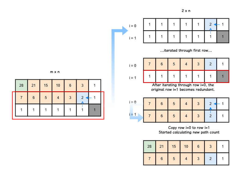
If you observe the recursive relation we’ve built so far (look at the traversal figure above), for any cell, the only cells needed are the one directly below it and the one directly to its right. So when declaring the array we only need a 2 x n array with m=2 (for Unique Paths, that’s all the space needed). So how do we store the path values this way?

The start here is still [m-2][n-2], i.e. step three’s second-to-last row and second-to-last column cell. You can think of it as taking the bottom two rows from the original m x n table and iterating as before. The iteration rule, as just mentioned, is that for any cell we only need the cell directly below and directly to its right. So for the first row (i=0) the rule is $F(m, n) = F(m+1, n) + F(m,n+1)$. Once the first row is computed, the second row used to compute it (which will all be 1 at first) has no further use, so we copy all the first row’s values into the second row to compute the new first row, following the same iteration rule. The final $F(0, 0)$ is then the overall path count.

class Solution {
public:
    int uniquePaths(int m, int n) {
        // init a m x n 2D vector with value 1
        vector<vector<int>> dp(2, vector<int>(n, 1));
        
        for(int i=m-2; i>=0; i--){
            for(int j=n-2; j>=0; j--){
                // Handloe first row
                // (m+n) = (cell below) + (cell on the right)
                dp[0][j] = dp[1][j] + dp[0][j+1];
            }
            // Move to second row
            dp[1] = dp[0];
        }
        return dp[0][0];
    }
};

Here we can compare the space complexity difference between step three and step four. Step three has to store the whole table, so its space complexity is $O(n \times m)$, while step four only stores $2*n$ cells, so its space complexity is $O(2 \times n) = O(n)$.

We can also observe the difference in the results:

Step three