🌐 中文版：繁體中文

Intro

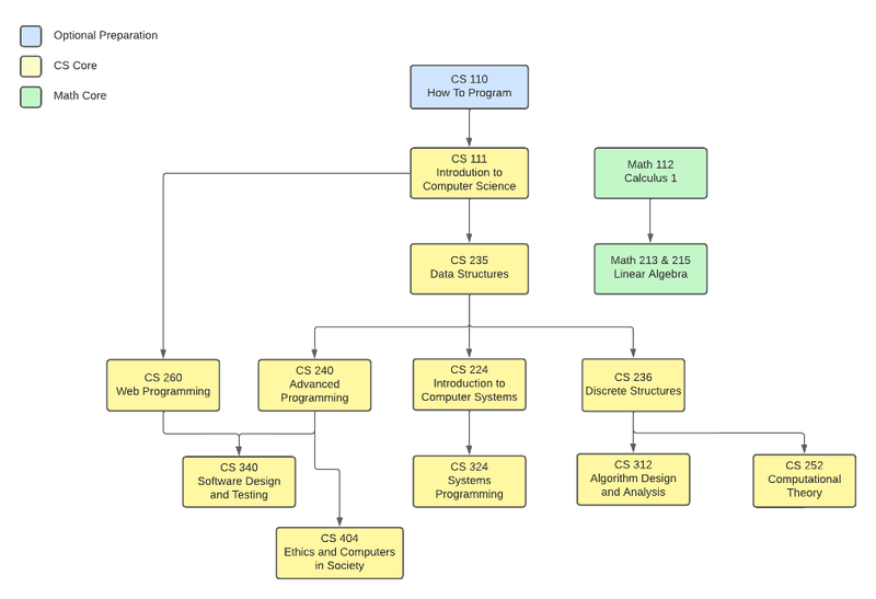
When we stored data before, common data structures were arrays, hash tables, linked lists, and so on. Imagine you’ve just started university and have a course schedule listing various courses in a table, but you don’t know which courses are prerequisites, which might be taken later, or which might block others. In this case, using a graph to represent the relationships between courses is very convenient. So one of the key points of a graph is preserving the relationships between pieces of data.

This blog post mainly references the explanation in this article

Definition of a Graph

Continuing the course graph above, each course represents a node, which can hold data, the data being the course name. And courses are connected by arrows, representing the relationships between courses.

vertex: each node in the graph is called a vertex, or node, and the set of all vertices is defined as $V$ or $V(G)$
edge: each line segment is called an edge. In a graph an edge is usually represented by a pair of vertices, $(V_{i}, V_{j})$ representing the edge between $V_{i}$ and $V_{j}$, and the set of all edges is usually defined as $E$ or $E(G)$

With $V$ and $E$ we can define what a graph is: the set of relationships between nodes, $G(V, E)$

Classification of graphs

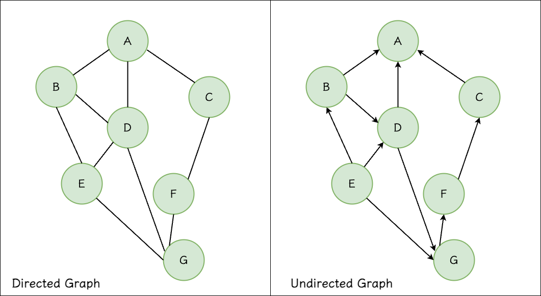
Graphs are mainly divided into Directed Graphs and Undirected Graphs based on whether the edges have direction

Directed Graph: the relationship between vertex(A) and vertex(B) is one-way, so the edge has direction; the set formed by all vertices and directional edges is a directed graph
Undirected Graph: the relationship between vertex(A) and vertex(B) is two-way, so the edge between them has no direction, and the set of vertices and edges formed is an undirected graph

Graph representations

So how do we represent a graph with a data structure? Common representations are the Adjacency Matrix and the Adjacency List.

Adjacency Matrix

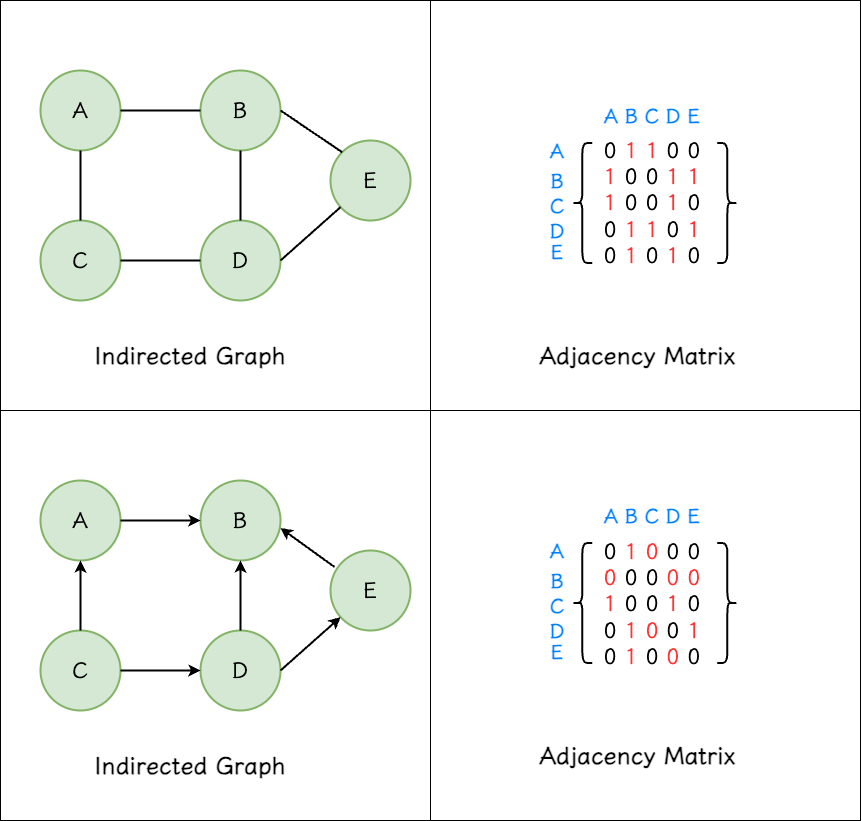
Let’s first look at the adjacency-matrix representation in an undirected graph: if there’s an edge between vertex(A) and vertex(B), then the positions corresponding to (A,B) and (B,A) are 1, and if there’s no edge between any two vertices, the matrix value is 0. For a directed graph, if there’s an edge from vertex(A) to vertex(B) but no edge from vertex(B) to vertex(A), then (A,B) is 1 but (B,A) is 0.

From the adjacency-matrix representation above you can also see that the adjacency matrix of an undirected graph is symmetric, while a directed graph’s is not. This also lets us deduce that transposing a directed graph’s matrix and overlaying it on the original matrix gives the undirected-graph representation.

Directed graph: $A[i][j]=1$ means there’s an edge from node i to node j
Undirected graph: $A[i][j]= A[j][i] = 1$ means there’s an undirected edge between node i and node j

With $A^T = A^{T}[i][j] = A[j][i]$ meaning there’s an edge from node j to node i. So $A_{undirected}[i][j] = A[i][j] V A[j][i]$

Adjacency List

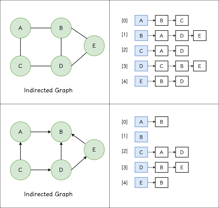
The adjacency-list representation first uses a one-dimensional array to represent all vertices, and for each array entry uses a linked list to represent the other vertices connected to it. Here, the order in which the linked list is connected doesn’t matter, because a graph is defined as a set. In the undirected graph above, taking vertex(D) as an example, it connects to vertex(C), vertex(B), vertex(E), so [3], i.e. vertex(D), can build a linked list connecting to vertex(C), vertex(B), vertex(E) (not necessarily in order). For a directed graph, vertex(D)’s linked list can only include nodes departing from vertex(D), i.e. vertex(B) and vertex(E).

Differences

	Adjacency Matrix	Adjacency List
Space complexity	$O(\lvert V \rvert^{2})$	$O( \lvert V \rvert + \lvert E \rvert)$
Notes	Good for dense graphs (many vertices and edges)	Good for sparse graphs (few edges)
Access	Contiguous memory is faster	Dynamic memory is slower
Add edge	Adding an edge just sets the corresponding position from 0 to 1, so $O(1)$	Adding a vertex to the front of the linked list is $O(1)$, but worst case is $O( \lvert E \rvert )$
Delete edge	Deleting an edge just changes the corresponding position from 1 to 0, so $O(1)$	Like deleting data in a linked list, $O( \lvert E \rvert)$

Adjacent: as long as there’s an edge between vertex(A) and vertex(B), they count as adjacent
Subgraph: for a $G’$, if the sets of edges and vertices composing it satisfy $V(G’)\subseteq V(G)$, $E(G’) \subseteq E(G)$, then $G’$ is a subgraph of $G$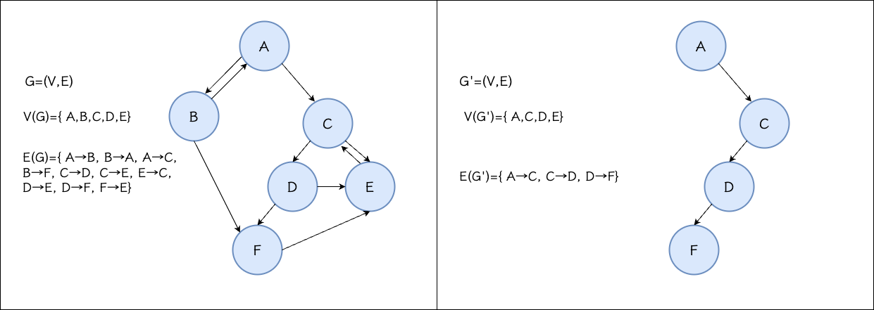

Path: the series of consecutively connected edges passed through from vertex(V1) to vertex(V2) is called the path from vertex(v1) to vertex(v2)
Length/Distance: the number of edges in a path
Simple path: if in a path, except for the start vertex and end vertex, all other vertices are passed through only once, then this path is a simple path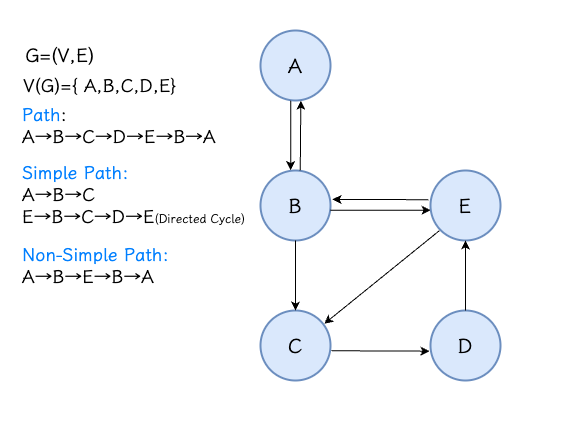

Cycle: if a simple path’s start vertex and end vertex are the same, this path is called a cycle. If the edges in the cycle are undirected, it’s an undirected cycle; if the cycle is traversed in order by direction, then the cycle is directed (directed cycle)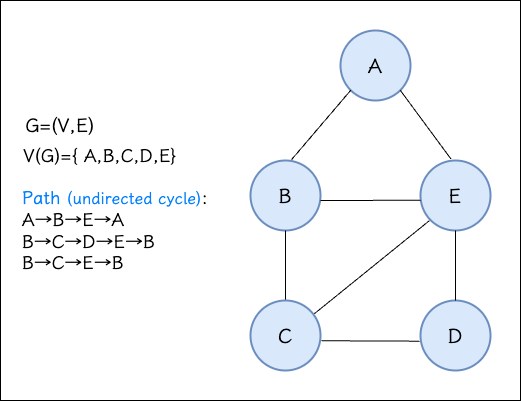

Acyclic graph: if there’s no cycle in a graph, the graph is called an acyclic graph. A tree is usually a kind of graph too, however if no simple path can be found in a tree whose start vertex and end vertex are the same, then the tree must be an acyclic graph

Weight: the weight, which can usually represent the distance or cost between two geographic locations. You can add a weight to an edge, and a graph with weights is called a weighted graph

Connected: what counts as two vertices being connected to each other? That’s being able to walk from vertex(A) to vertex(B) and from vertex(B) to vertex(A). So for an undirected graph, that’s vertex(A) and vertex(B) being connected by an edge, and for a directed graph, that’s the existence of edge(A→B) as well as edge(B→A)

Connected in undirected graph: for an undirected graph, if any vertex has a path connecting to the others, then this undirected graph is called connected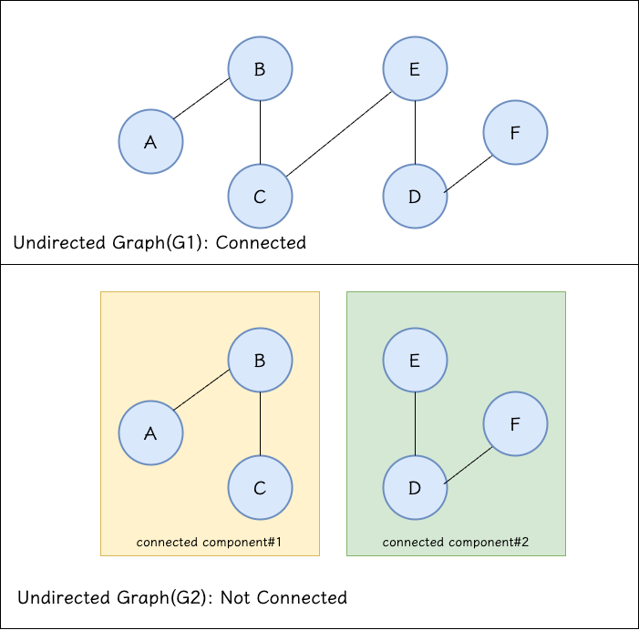

Connected components: in an undirected graph, there’s some subgraph that is connected, and if adding other vertices or edges would break this connected property, then this subgraph is called a connected component. Both subgraphs at the bottom of the figure above satisfy this property.

Strongly connected in directed graph: in a directed graph, for any two vertices vertex(A) and vertex(B), there exist both (1) a path from vertex(A) to vertex(B) and (2) a path from vertex(B) to vertex(A). Then this directed graph is called strongly connected

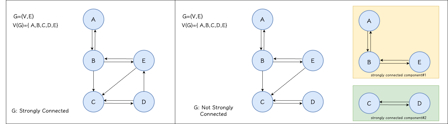
Strongly connected component: in a directed graph, there’s some subgraph that is strongly connected, and if adding other vertices or edges would break this strongly connected property, then this subgraph is called a strongly connected component. (The maximal set that maintains being connected.)

Self-loop: if there’s an edge from vertex(A) to vertex(A), it’s a self-loop

Graph application scenarios

Graphs are mainly used in scenarios like the Minimum Spanning Tree (MST), network flow, and shortest-path problems. Before applying them to a scenario, you first need to know the methods for searching vertices in a graph.